| Mehdi Shadkhah | Ronak Tali | Ali Rabeh | Ethan Herron | Cheng-Hau Yang | Abhisek Upadhyaya |
| Iowa State University | Iowa State University | Iowa State University | Iowa State University | Iowa State University | New York University |
| Ames, IA, USA | Ames, IA, USA | Ames, IA, USA | Ames, IA, USA | Ames, IA, USA | New York, NY, USA |
| Adarsh Krishnamurthy | Chinmay Hegde | Aditya Balu | Baskar Ganapathysubramanian |
| Iowa State University | New York University | Iowa State University | Iowa State University |
| Ames, IA, USA | New York, NY, USA | Ames, IA, USA | Ames, IA, USA |
| 2D | 3D |
In MPF-Bench dataset, we present a comprehensive collection of simulations designed to capture the intricate physics of falling droplets in both two-dimensional and three-dimensional settings. The Droplet-2D dataset includes 5,000 simulations with each simulation providing 101 time steps, offering a detailed view of how various fluid properties, such as density and viscosity ratios, influence the behavior of droplets as they fall under gravity. In contrast, the Droplet-3D dataset, though smaller with 500 simulations and 51 time steps per simulation, provides a three-dimensional perspective on the same phenomena, allowing for a more nuanced understanding of the complex interactions between forces like gravity and surface tension. Both datasets are generated using the Lattice Boltzmann method, ensuring high fidelity in capturing the droplet dynamics, including deformation and breakup, across a wide range of Reynolds and Bond numbers. These datasets are a critical resource for training and validating Scientific Machine Learning (SciML) models, enabling more accurate predictions of multiphase flow behavior in various engineering and scientific applications.
| 2D | 3D |
The Bubble dataset in MPF-Bench is an extensive collection of simulations that captures the dynamic behavior of rising bubbles in both two-dimensional and three-dimensional environments. The Bubble-2D dataset includes 5,000 simulations, each comprising 101 time steps, providing a detailed exploration of bubble dynamics under varying fluid properties, such as density and viscosity ratios. These simulations illustrate how bubbles rise through a denser fluid medium, influenced by factors like buoyancy and surface tension, leading to complex phenomena such as shape deformation and breakup. The Bubble-3D dataset, consisting of 500 simulations with 51 time steps each, offers a three-dimensional perspective, allowing for a more intricate examination of bubble behavior, including oscillations and path instability. Both datasets are generated using the Lattice Boltzmann method, ensuring high accuracy in capturing the essential physics of bubble dynamics across a wide range of Reynolds and Bond numbers. These datasets are instrumental for developing and testing Scientific Machine Learning (SciML) models, which aim to improve the prediction and understanding of multiphase flow phenomena in various scientific and industrial applications.
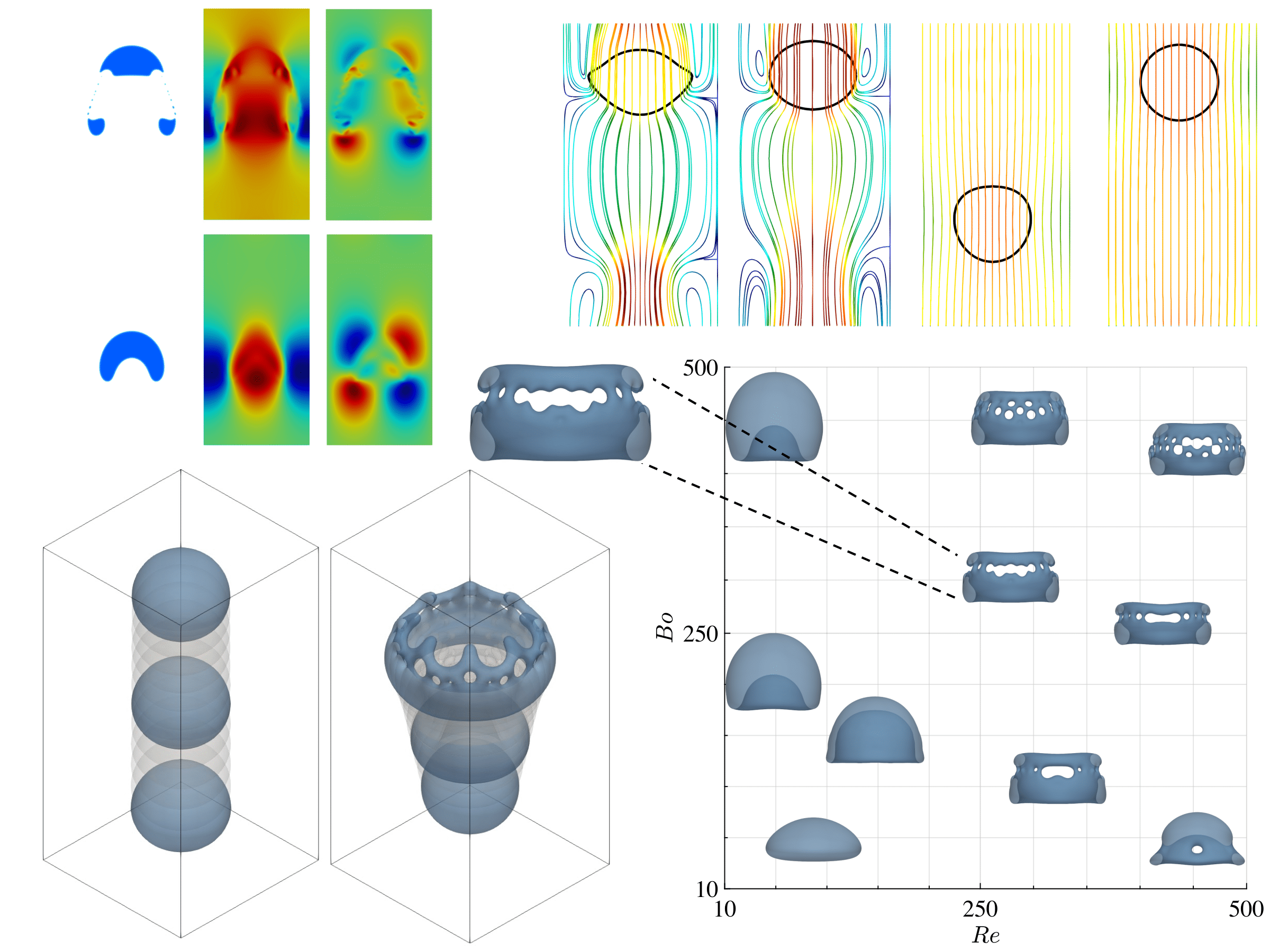
In fluid dynamics, the Reynolds number (Re) and Bond number (Bo) are two critical dimensionless quantities that characterize the flow regime of two-phase systems such as bubbles and droplets. The Reynolds number, Re, is a measure of the ratio of inertial forces to viscous forces within the fluid, and it indicates whether the flow will be laminar or turbulent. The Bond number, Bo, on the other hand, represents the ratio of gravitational forces to surface tension forces, determining the shape and stability of bubbles or droplets in a fluid.
MPF-Bench dataset spans a wide range of these two parameters, capturing multiple flow regimes from simple, predictable behaviors to highly complex, turbulent ones. The accompanying figure showcases four distinct cases from the 3D bubble dataset, highlighting scenarios with both low and high Reynolds and Bond numbers. As these numbers increase, the bubble undergoes significant deformation, making it more challenging for models to accurately predict its behavior. This trend is also observed in droplet dynamics, where increased Re and Bo lead to more intricate and harder-to-predict flows. By understanding the flow regimes represented in our dataset, users can better choose between easier or more challenging cases to train and assess their models, depending on their specific research or application needs.
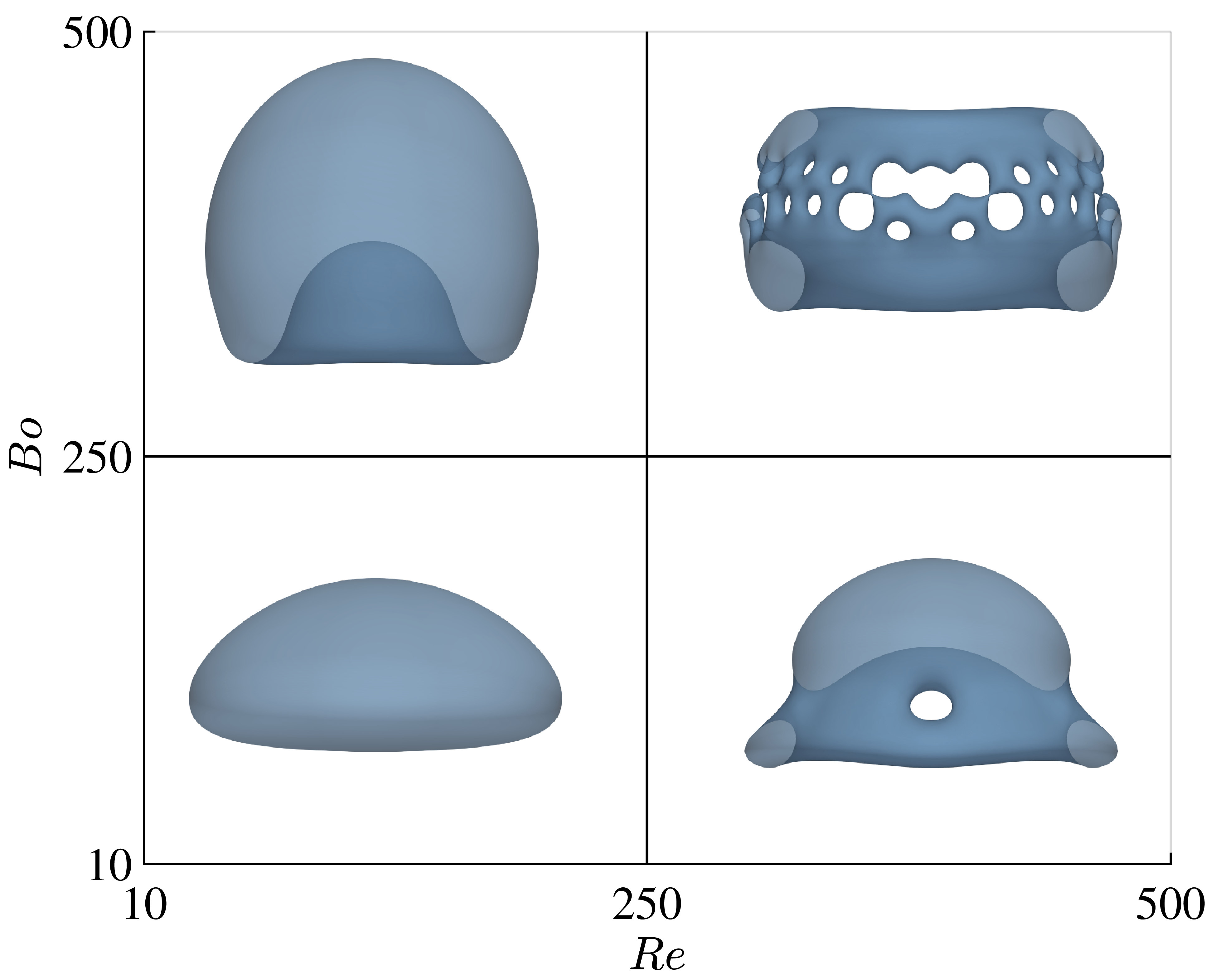
Figure: Visualization of four different cases from the 3D bubble dataset, illustrating the impact of varying Reynolds (Re) and Bond (Bo) numbers on bubble deformation. As Re and Bo numbers increase, the bubble exhibits more complex and challenging dynamics, demonstrating the varying levels of difficulty in predicting bubble behavior across different flow regimes.
We provide a comprehensive table to help users select the most suitable cases for training and evaluating their models. Our dataset includes variations in key parameters, such as the Reynolds number (Re), Rho Ratio, Viscosity Ratio, and Bond Number (Bo). The Rho Ratio ranges from 10 to 1000, Viscosity Ratio varies between 1 and 100, and the Bo number spans from 10 to 500. Notably, the Reynolds number in bubble simulations varies from 10 to 500, while in drop simulations, it extends from 10 to 1000. Due to the inherent fluid properties, the Viscosity Ratio is proportional to the Density Ratio, meaning that both are typically either high or low together. To support model development, we have introduced a normalized difficulty classification that reflects the complexity of capturing interface deformations. This relative difficulty rating guides users in selecting cases, with most scenarios following this established pattern.
| Density Ratio | Viscosity Ratio | \(Bo\) Number | \(Re\) Number | Difficulty |
|---|---|---|---|---|
| High | High | High | High | Challenging |
| High | High | Low | Low | Easy |
| High | High | High | Low | Moderate |
| High | High | Low | High | Moderate |
| Low | Low | High | High | Challenging |
| Low | Low | Low | Low | Easy |
| Low | Low | High | Low | Easy |
| Low | Low | Low | High | Moderate |
MPF-Bench dataset is extensive, comprising a total of 11,000 simulations divided equally between bubble and droplet dynamics, with each category further broken down into 2D and 3D simulations. For both 2D and 3D simulations, we provide detailed input parameters, including the density ratio, viscosity ratio, Reynolds number, and Bond number. These inputs are critical in determining the complex flow behaviors captured in the dataset. The outputs of our simulations include key fields such as the interface indicator, velocity components in all directions, pressure, and density, which provide a comprehensive view of the multiphase flow dynamics. The dataset is structured in a way that allows for easy integration into Scientific Machine Learning (SciML) models, facilitating advancements in the understanding and prediction of multiphase flow phenomena.
| Dataset | Dim. | Input Tensor | Output Tensor | Size of Dataset (GB) |
|---|---|---|---|---|
| Droplet | 2D | X[5000][\(\rho^*\), \(\mu^*\), Bo, Re] | Y [5000][101][c, u, v, p, \(\rho\)][y][x] | 566 GB |
| Bubble | 2D | X[5000][\(\rho^*\), \(\mu^*\), Bo, Re] | Y [5000][101][c, u, v, p, \(\rho\)][y][x] | 822 GB |
| Droplet | 3D | X[500][\(\rho^*\), \(\mu^*\), Bo, Re] | Y [500][51][c, u, v, w, p, \(\rho\)][z][y][x] | 1200 GB |
| Bubble | 3D | X[500][\(\rho^*\), \(\mu^*\), Bo, Re] | Y [500][51][c, u, v, w, p, \(\rho\)][z][y][x] | 1400 GB |
To facilitate easier access and experimentation with our extensive dataset, we have provided a down-sampled version. This sample dataset is specifically tailored for quick testing and prototyping, containing 100 simulations for each of the 2D categories and 5 simulations for each of the 3D categories. Each of these simulations is further simplified, with only 10 time steps included. This allows users to get a taste of the full dataset's capabilities without the need for extensive computational resources or time commitment. The down-sampled dataset serves as an excellent starting point for researchers and developers to explore the dynamics of droplet and bubble behaviors in both 2D and 3D, making it easier to test ideas and methodologies before scaling up to the full dataset.
Proposed in 2015 for image segmentation tasks, UNet is designed around the concept of semantic segmentation—assigning a class to every pixel in an image. It achieves this through a series of encoders and decoders, connected by bridge blocks, arranged in a sequential and symmetrical pattern that resembles the shape of the letter "U," which is where the name UNet comes from. One of the key advantages of UNet is its ability to extract the maximum amount of information from each image, enabling it to perform as well as traditional convolutional neural networks in image classification tasks, but with significantly fewer training samples.
Reference: Ronneberger, O., Fischer, P., & Brox, T. (2015). U-Net: Convolutional Networks for Biomedical Image Segmentation. In Medical Image Computing and Computer-Assisted Intervention -- MICCAI 2015 (pp. 234-241). Springer International Publishing.
Proposed in 2019, DeepONets are based on the Universal Approximation Theorem for operators. The core idea is to split the problem into two parts: the input function evaluations at specific locations are passed through a fully connected neural network called the branch net, while the location coordinates where outputs are desired are passed through another fully connected network called the trunk net. The outputs from these two networks are then combined through a dot product, which is compared with the actual outputs during training. The entire system is trained using a loss function and backpropagation. One of the appealing aspects of DeepONet is its simplicity; it doesn’t require complex hyperparameter tuning, as fairly general fully connected networks with a few hidden layers work effectively for most cases.
Reference: Lu, L., Jin, P., Pang, G., Zhang, Z., & Karniadakis, G. E. (2021). Learning nonlinear operators via DeepONet based on the universal approximation theorem of operators. Nature Machine Intelligence, 3, 218–229.
Proposed in 2020, the Fourier Neural Operator (FNO) is a neural operator designed to approximate continuous nonlinear operator solutions to partial differential equations (PDEs). It achieves this by stacking a sequence of linear integral operators, which are implemented using a combination of convolutional kernels and the Fast Fourier Transform (FFT). After applying FFT, high frequencies are truncated to respect the Nyquist limit, and then an Inverse Fast Fourier Transform (IFFT) is applied. This process is followed by nonlinear activation functions, creating a block that forms the core of the FNO architecture. For practitioners, several hyperparameters are crucial when working with FNOs: the number of operator blocks, the number of retained frequencies after FFT, and the number of hidden nodes.
Reference: Li, Z., Kovachki, N., Azizzadenesheli, K., Liu, B., Bhattacharya, K., Stuart, A., & Anandkumar, A. (2021). Fourier Neural Operator for Parametric Partial Differential Equations. arXiv preprint arXiv:2010.08895.
Proposed in 2023, the Convolutional Neural Operator (CNO) is an adaptation of the U-Net architecture specifically designed for operator learning. CNOs address a common issue found in Fourier Neural Operators (FNOs), where the application of nonlinearity can cause an explosion in the frequency spectrum, leading to violations of the Nyquist barrier. CNOs mitigate this problem through a carefully structured series of upsampling, downsampling, and residual blocks, which allow them to maintain a structure-preserving operator that satisfies the property of Continuous-Discrete Equivalence. When working with CNOs, the two primary hyperparameters to tune are the number of upsampling/downsampling blocks and the learning rate for the optimizer.
Reference: Raonić, B., Molinaro, R., De Ryck, T., Rohner, T., Bartolucci, F., Alaifari, R., Mishra, S., & de Bézenac, E. (2023). Convolutional Neural Operators for robust and accurate learning of PDEs. arXiv preprint arXiv:2302.01178.
Proposed as a foundation model for scientific machine learning, Poseidon is based on the Scalable Operator Transformers (scOT) architecture, which combines hierarchical, multiscale vision transformers with U-Net-style encoder-decoder structures. Specifically, it integrates Swin Transformer V2 blocks with ConvNeXt residual blocks to capture multiscale dependencies efficiently. Trained on a large dataset of compressible Euler and incompressible Navier-Stokes equations, Poseidon is designed to generalize across complex fluid dynamics scenarios. The model is available in three sizes—tiny (20M parameters), base (160M parameters), and large (630M parameters). In this work, we utilize the tiny version of Poseidon (Poseidon-T), which provides a balance between computational efficiency and predictive accuracy for our experiments.
Reference: Herde, M., Raonić, B., Rohner, T., Käppeli, R., Molinaro, R., de Bézenac, E., & Mishra, S. (2024). Poseidon: Efficient foundation models for PDEs.
The Sequence to Field evaluation tests how well machine learning models predict the interface field C of multiphase flows
given different input sequences. We set up three different data subsets: S1, S2, and S3. The models receive either a single timestep t1,
sequences from t1 to t3, or sequences from t1 to t5, and they predict the corresponding next time snapshot
for each subset. The figure below compares the ground truth with predictions from UNet, CNO, DeepONet, and Poseidon, where each row represents a different subset.
S1 corresponds to a simpler case with minimal deformation, S2 involves moderate interface changes, and S3 represents a more challenging case
with significant interface deformation. CNO achieves the best performance, maintaining accurate interface structures, while DeepONet struggles with high-deformation cases.
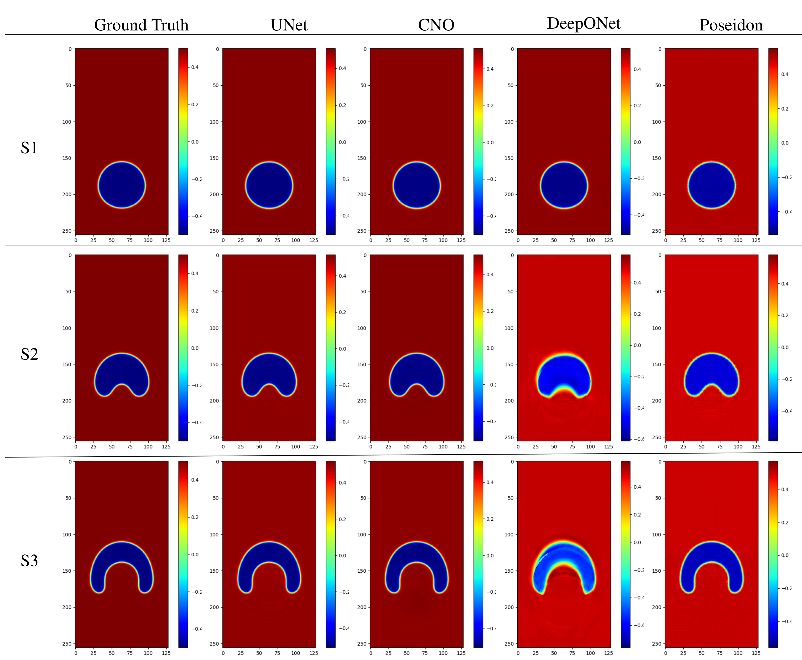
Figure: The figure presents a comparison of sequence-to-field predictions for the concentration field C against the ground truth. The predictions are generated by four models: UNet, Convolutional Neural Operator (CNO), DeepONet, and Poseidon, across three data subsets (S1, S2, and S3). Each row corresponds to a different subset (S1, S2, or S3), while each column displays the predictions made by the respective models.
| Model | Channel | S1 | S2 | S3 | |||
|---|---|---|---|---|---|---|---|
| MSE | \(L_2\) | MSE | \(L_2\) | MSE | \(L_2\) | ||
| UNet | \(c\) | 2.60 × 10⁻² | 2.59 × 10⁻² | 8.40 × 10⁻³ | 8.07 × 10⁻³ | 9.56 × 10⁻³ | 9.04 × 10⁻³ |
| \(u\) | 8.80 × 10⁻⁵ | 3.13 × 100 | 8.00 × 10⁻⁶ | 2.04 × 100 | 1.00 × 10⁻⁵ | 2.09 × 100 | |
| \(v\) | 1.00 × 10⁻⁶ | 1.56 × 100 | 1.00 × 10⁻⁶ | 7.84 × 10⁻¹ | 1.00 × 10⁻⁶ | 8.76 × 10⁻¹ | |
| \(p\) | 1.00 × 10⁻⁶ | 2.74 × 10² | 1.00 × 10⁻⁶ | 3.23 × 10² | 1.00 × 10⁻⁶ | 5.17 × 10² | |
| DeepONet | \(c\) | 2.66 × 10⁻² | 2.65 × 10⁻² | 1.01 × 10⁻¹ | 1.01 × 10⁻¹ | 1.18 × 10⁻¹ | 1.18 × 10⁻¹ |
| \(u\) | 9.10 × 10⁻⁵ | 6.71 × 100 | 1.27 × 10⁻³ | 1.24 × 100 | 1.71 × 10⁻³ | 9.18 × 10⁻¹ | |
| \(v\) | 1.00 × 10⁻⁶ | 8.68 × 10⁻¹ | 1.00 × 10⁻⁶ | 5.35 × 10⁻¹ | 1.00 × 10⁻⁶ | 8.89 × 10⁻¹ | |
| \(p\) | 1.00 × 10⁻⁶ | 1.89 × 10² | 1.00 × 10⁻⁶ | 2.43 × 10² | 1.00 × 10⁻⁶ | 1.66 × 10² | |
| FNO | \(c\) | 2.72 × 10⁻² | 2.68 × 10⁻² | 9.73 × 10⁻³ | 8.97 × 10⁻³ | 2.10 × 10⁻² | 1.98 × 10⁻² |
| \(u\) | 9.30 × 10⁻⁵ | 8.56 × 100 | 1.00 × 10⁻⁵ | 2.77 × 100 | 4.80 × 10⁻⁵ | 5.29 × 100 | |
| \(v\) | 1.00 × 10⁻⁶ | 3.43 × 100 | 1.00 × 10⁻⁶ | 1.09 × 100 | 2.00 × 10⁻⁶ | 2.02 × 100 | |
| \(p\) | 1.00 × 10⁻⁶ | 7.18 × 10² | 1.00 × 10⁻⁶ | 7.44 × 10² | 2.00 × 10⁻⁶ | 1.04 × 10³ | |
| CNO | \(c\) | 2.62 × 10⁻² | 2.60 × 10⁻¹ | 5.89 × 10⁻³ | 5.65 × 10⁻³ | 9.41 × 10⁻³ | 9.00 × 10⁻³ |
| \(u\) | 8.80 × 10⁻⁵ | 5.04 × 100 | 4.00 × 10⁻⁶ | 1.60 × 100 | 1.00 × 10⁻⁵ | 1.79 × 100 | |
| \(v\) | 1.00 × 10⁻⁶ | 1.73 × 100 | 1.00 × 10⁻⁶ | 5.07 × 10⁻¹ | 1.00 × 10⁻⁶ | 9.19 × 10⁻¹ | |
| \(p\) | 1.00 × 10⁻⁶ | 4.46 × 10² | 1.00 × 10⁻⁶ | 2.24 × 10² | 1.00 × 10⁻⁶ | 3.96 × 10² | |
| scOT | \(c\) | 2.76 × 10⁻² | 2.68 × 10⁻² | 1.77 × 10⁻² | 1.68 × 10⁻² | 2.23 × 10⁻² | 2.17 × 10⁻² |
| \(u\) | 1.29 × 101 | 1.29 × 101 | 3.50 × 10⁻⁵ | 3.91 × 100 | 5.80 × 10⁻⁵ | 2.82 × 100 | |
| \(v\) | 5.24 × 100 | 5.24 × 100 | 1.00 × 10⁻⁶ | 2.31 × 100 | 1.00 × 10⁻⁶ | 1.75 × 100 | |
| \(p\) | 9.65 × 10² | 9.65 × 10² | 2.00 × 10⁻⁶ | 8.12 × 10² | 2.00 × 10⁻⁶ | 7.80 × 10² | |
| Poseidon | \(c\) | 2.87 × 10⁻² | 2.79 × 10⁻¹ | 3.01 × 10⁻² | 2.49 × 10⁻² | 2.49 × 10⁻² | 2.23 × 10⁻² |
| \(u\) | 1.00 × 10⁻⁴ | 1.16 × 101 | 1.14 × 10⁻⁴ | 1.31 × 101 | 6.10 × 10⁻⁵ | 8.28 × 100 | |
| \(v\) | 2.00 × 10⁻⁶ | 5.86 × 100 | 1.00 × 10⁻⁶ | 4.05 × 100 | 5.00 × 10⁻⁶ | 2.83 × 100 | |
| \(p\) | 2.00 × 10⁻⁶ | 1.04 × 10³ | 6.00 × 10⁻⁶ | 2.35 × 10³ | 4.00 × 10⁻⁶ | 1.94 × 10³ | |
The Sequence to Sequence evaluation extends the challenge by predicting a sequence of future states rather than a single snapshot.
The models are trained on past sequences and tasked with predicting the system's evolution at three consecutive time steps. We define three test cases:
S4, S5, and S6, where input sequences range from t1 to t3, t1 to t5, and t1 to t8, respectively.
The figure below compares predictions from different models against ground truth at key time steps T9, T10, and T11, showing how well each model maintains accuracy over time.
CNO again performs best, accurately capturing complex interface dynamics, while DeepONet exhibits increasing errors, particularly in high-deformation regions.
This benchmark provides insights into how well neural operators forecast long-term fluid dynamics.
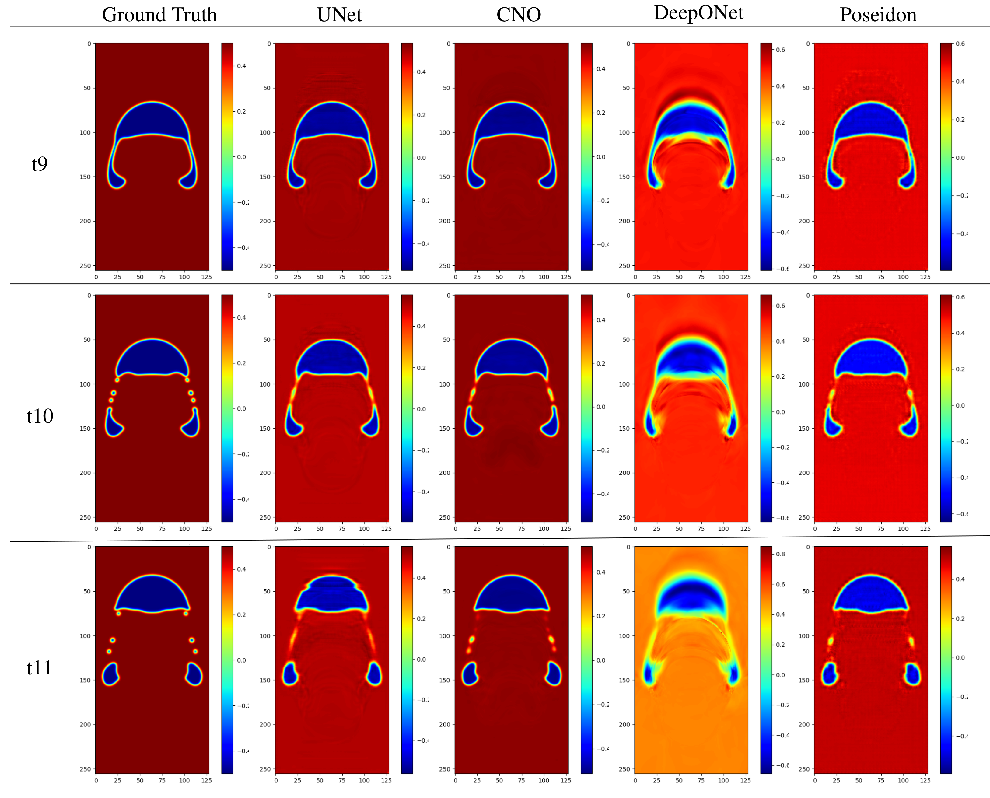
Figure: The figure presents sequence-to-sequence predictions for the concentration field C compared to the ground truth. Predictions are made by four models: UNet, Convolutional Neural Operator (CNO), DeepONet, and Poseidon. Each row represents different time steps (t9, t10, and t11) from dataset S6, while each column shows the predictions from the respective models.
| Model | Channel | S4 | S5 | S6 | |||
|---|---|---|---|---|---|---|---|
| MSE | \(L_2\) | MSE | \(L_2\) | MSE | \(L_2\) | ||
| UNet | \(c\) | 3.27 × 10⁻² | 2.87 × 10⁻² | 3.93 × 10⁻² | 3.31 × 10⁻² | 7.34 × 10⁻² | 6.58 × 10⁻² |
| \(u\) | 1.35 × 10⁻⁴ | 3.54 × 100 | 2.02 × 10⁻⁴ | 3.10 × 100 | 6.65 × 10⁻⁴ | 3.90 × 100 | |
| \(v\) | 1.00 × 10⁻⁶ | 1.38 × 100 | 1.00 × 10⁻⁶ | 1.45 × 100 | 1.00 × 10⁻⁶ | 9.54 × 10⁻¹ | |
| \(p\) | 1.00 × 10⁻⁶ | 6.76 × 10² | 1.00 × 10⁻⁶ | 6.30 × 10² | 1.00 × 10⁻⁶ | 7.79 × 10² | |
| DeepONet | \(c\) | 1.64 × 10⁻¹ | 1.60 × 10⁻¹ | 2.03 × 10⁻¹ | 1.99 × 10⁻¹ | 1.94 × 10⁻¹ | 1.92 × 10⁻¹ |
| \(u\) | 3.33 × 10⁻³ | 3.15 × 100 | 5.04 × 10⁻³ | 1.64 × 100 | 4.57 × 10⁻³ | 1.32 × 100 | |
| \(v\) | 1.00 × 10⁻⁶ | 1.04 × 100 | 1.00 × 10⁻⁶ | 7.59 × 10⁻¹ | 1.00 × 10⁻⁶ | 3.83 × 10⁻¹ | |
| \(p\) | 1.00 × 10⁻⁶ | 7.30 × 10² | 1.00 × 10⁻⁶ | 3.53 × 10² | 1.00 × 10⁻⁶ | 3.17 × 10² | |
| FNO | \(c\) | 1.16 × 10⁻² | 1.10 × 10⁻² | 2.33 × 10⁻² | 2.20 × 10⁻² | 4.24 × 10⁻² | 4.00 × 10⁻² |
| \(u\) | 1.70 × 10⁻⁵ | 1.00 × 100 | 6.50 × 10⁻⁵ | 2.98 × 100 | 2.28 × 10⁻⁴ | 1.13 × 100 | |
| \(v\) | 1.00 × 10⁻⁶ | 4.50 × 10⁻¹ | 1.00 × 10⁻⁶ | 1.28 × 100 | 1.00 × 10⁻⁶ | 3.98 × 10⁻¹ | |
| \(p\) | 1.00 × 10⁻⁶ | 1.38 × 10² | 1.00 × 10⁻⁶ | 7.87 × 10² | 1.00 × 10⁻⁶ | 2.69 × 10² | |
| CNO | \(c\) | 1.74 × 10⁻² | 1.69 × 10⁻² | 1.72 × 10⁻² | 1.63 × 10⁻² | 3.78 × 10⁻² | 3.53 × 10⁻² |
| \(u\) | 3.70 × 10⁻⁵ | 1.51 × 100 | 3.60 × 10⁻⁵ | 1.37 × 100 | 1.76 × 10⁻⁴ | 1.74 × 100 | |
| \(v\) | 1.00 × 10⁻⁶ | 6.87 × 10⁻¹ | 1.00 × 10⁻⁶ | 6.85 × 10⁻¹ | 1.00 × 10⁻⁶ | 5.98 × 10⁻¹ | |
| \(p\) | 1.00 × 10⁻⁶ | 2.84 × 10² | 1.00 × 10⁻⁶ | 2.93 × 10² | 1.00 × 10⁻⁶ | 4.22 × 10² | |
| scOT | \(c\) | 3.85 × 10⁻³ | 3.69 × 100 | 3.79 × 10⁻³ | 6.27 × 100 | 6.27 × 10⁻³ | 5.79 × 100 |
| \(u\) | 1.73 × 10⁻⁴ | 6.73 × 100 | 6.73 × 100 | 5.73 × 100 | 4.85 × 10⁻⁴ | 5.31 × 100 | |
| \(v\) | 3.00 × 10⁻⁶ | 2.78 × 100 | 3.00 × 10⁻⁶ | 2.12 × 100 | 2.00 × 10⁻⁶ | 1.93 × 100 | |
| \(p\) | 3.00 × 10⁻⁶ | 1.48 × 10³ | 3.00 × 10⁻⁶ | 1.34 × 10³ | 1.00 × 10⁻⁶ | 1.21 × 10³ | |
| Poseidon | \(c\) | 3.06 × 10⁻² | 2.84 × 100 | 3.33 × 10⁻² | 3.17 × 10⁻² | 5.99 × 10⁻² | 5.79 × 10⁻¹ |
| \(u\) | 1.01 × 10⁻⁴ | 8.26 × 100 | 1.26 × 10⁻⁴ | 6.49 × 100 | 4.30 × 10⁻⁴ | 7.79 × 100 | |
| \(v\) | 5.00 × 10⁻⁶ | 3.51 × 100 | 4.00 × 10⁻⁶ | 2.47 × 100 | 5.00 × 10⁻⁶ | 2.16 × 100 | |
| \(p\) | 5.00 × 10⁻⁶ | 1.71 × 10³ | 4.00 × 10⁻⁶ | 1.48 × 10³ | 5.00 × 10⁻⁶ | 1.81 × 10³ | |
All models were trained on a single A100 80GB GPU, batch size of 4, Adam optimizer with learning rate of 10^−3, and run for 400 epochs. The shown validation loss for CNO sequence to field prediction on the bubble dataset seems to saturate after 300 epochs. Similar behavior is demonstrated by the other networks.
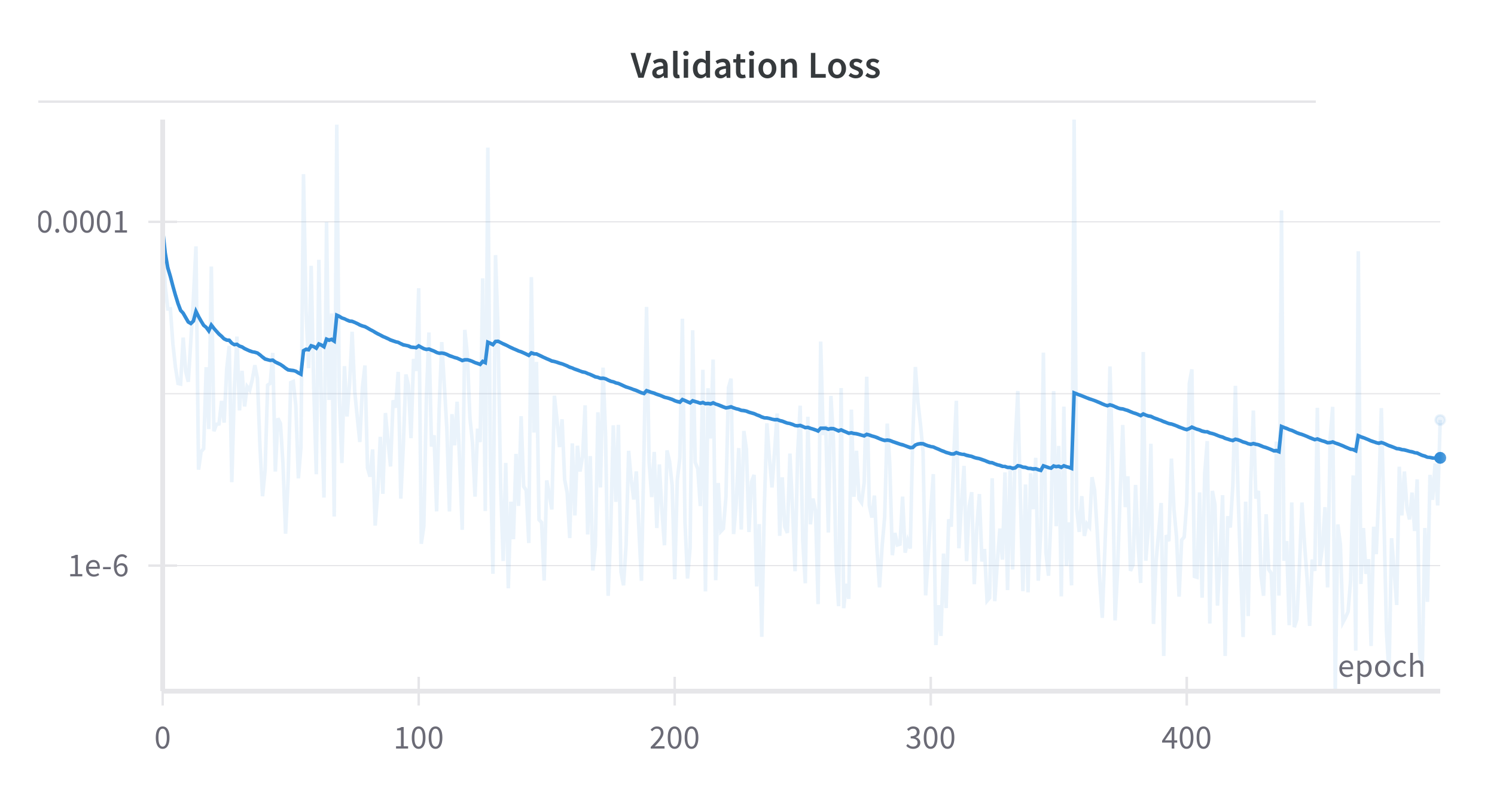
Figure: Validation Loss Curve: This plot illustrates the decline in validation loss over the course of training epochs, indicating the model's performance and improvement during the training process.
These dataset subsets contains all samples used in our paper, specifically for the results presented in the publication. Anyone interested in reproducing our results or benchmarking their methods can use this exact subset. While the full dataset is much larger, this selection includes all the data points referenced in our analysis and figures.
 Paper
Paper GitHub
 Dataset